Volumetric Data on a Three-Dimensional Grid

Cube Files

Store atomic coordinates and scalar values on a three-dimensional grid to connect electronic-structure calculations, real-space analysis, and visualization.

Role: Exchange format for 3D fields
Typical input: Density, MO, ESP, spin density, RDG
Typical output: ASCII grid and molecular geometry

1. What a cube file stores

A cube file is a container, not a physical observable. Its values may represent electron density, a molecular orbital, electrostatic potential, spin density, or an analysis field. Save the field definition and generation command with the file.

The extension does not identify the field

A .cube file may contain a density, orbital amplitude, potential, or derived function. Preserve the field definition, units, method, orbital number, and generation command.

2. File structure

The format contains two comment lines, atom count and grid origin, three grid axes, atom records, and voxel values. Axis vectors need not be parallel to the Cartesian axes.

Cube skeleton

comment line 1
comment line 2
N_atoms  origin_x origin_y origin_z
N_x      dx_x dx_y dx_z
N_y      dy_x dy_y dy_z
N_z      dz_x dz_y dz_z
Z_1      q_1  x_1 y_1 z_1
...
voxel values

Voxel values are conventionally written with the z index changing fastest. Confirm that the number of values equals Nx * Ny * Nz; some variants store multiple orbitals and require additional header information.

3. Grid coordinates and units

r (i, j, k) = r_{0} + i a_{1} + j a_{2} + k a_{3}

Confirm the producer's unit convention. Halving the spacing approximately doubles each dimension and increases the total voxel count about eightfold.

Gaussian-style files usually use atomic units, while some readers interpret negative voxel counts as an Angstrom convention. Do not infer units from appearance; check the producer and reader specifications.

4. Physical fields

Field	Important property
Electron density	Normally nonnegative; its integral relates to electron count
Molecular orbital	Signed amplitude, not an electron density
Spin density	Difference between alpha and beta densities
Electrostatic potential	Often mapped onto a density isosurface

An orbital's global sign has no physical meaning. Before subtracting or comparing orbital cubes from separate calculations, match orbitals and align their phases.

5. Generation

Gaussian uses formchk and cubegen; PySCF provides pyscf.tools.cubegen; ORCA uses %plots or orca_plot; Multiwfn can export many wavefunction-derived fields.

PySCF

from pyscf.tools import cubegen

dm = mf.make_rdm1()
cubegen.density(mol, "density.cube", dm, resolution=0.20)
cubegen.mep(mol, "esp.cube", dm, resolution=0.20)

formchk job.chk job.fchk
cubegen 0 density=scf job.fchk density.cube -2 h
cubegen 0 MO=Homo job.fchk homo.cube -2 h

6. Arithmetic on cube data

Pointwise differences require identical origins, axis vectors, shapes, units, geometries, and field definitions.

Δρ (r) = ρ_{AB} - ρ_{A} - ρ_{B}

Prefer regeneration to interpolation

Generate all fields on the same explicit grid whenever possible. Interpolation introduces numerical and boundary errors.

7. Visualization and validation

Use equal positive and negative isovalues for signed orbitals, fixed color ranges for comparisons, and record every isovalue. Verify voxel count, margins, field integrals where applicable, and the mapping between geometry and field.

Continue to Multiwfn, NCIplot, or py3Dmol.

8. Numerical validation

Confirm field identity, method, orbital index, and units.
Compare header dimensions with the number of voxel values.
Check that the molecule is not clipped by the grid boundary.
For density, multiply the numerical sum by the voxel volume and compare with the electron count.
For arithmetic, compare origin, axes, shape, geometry, and units programmatically.

Reproducible Example

9. Calculated example: acetone cube fields

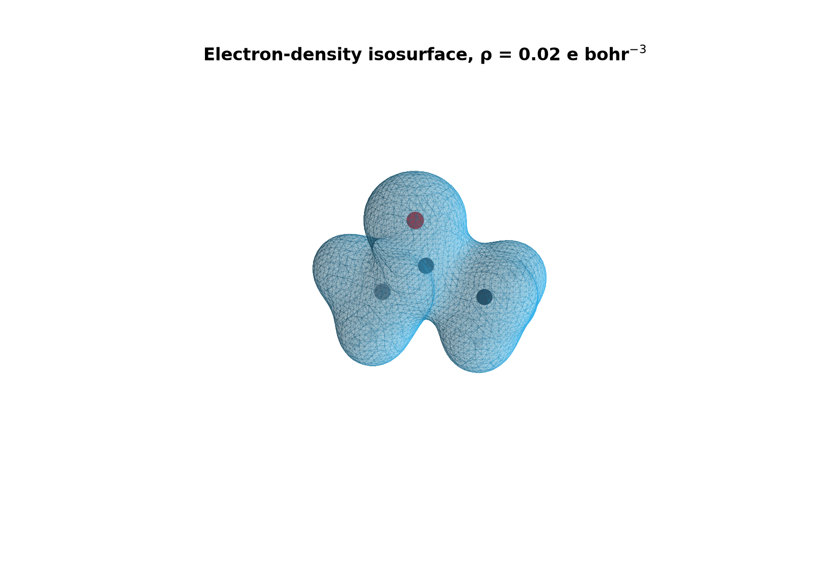
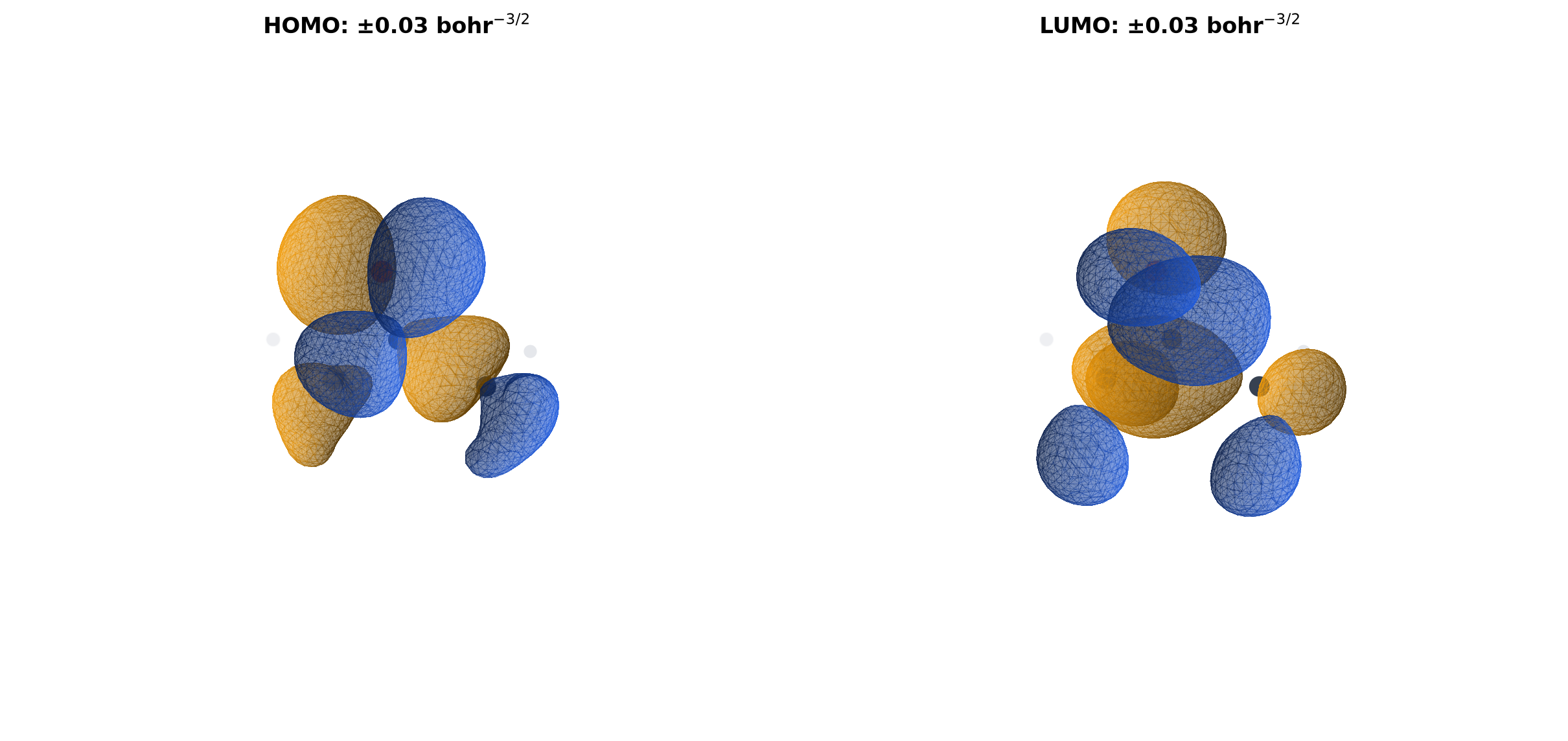
An RDKit-prepared acetone geometry was used for a PySCF 2.14.0 B3LYP/def2-SVP single-point calculation, with 0.24 Å spacing and a 4.0 Å margin.

SCFConverged

Total energy-193.01179457 E_h

HOMO / LUMO-0.24841 / -0.01895 E_h

Density integral32.0389 e (expected 32)

Loading cube data...

Translucent cyan: electron density at ρ = 0.02 e bohr^-3.

Drag to rotate. ESP colors the density isosurface using the separate ESP cube. 3Dmol.js 2.5.5

Acetone electron-density isosurface — Electron density at ρ = 0.02 e bohr^-3.

Acetone HOMO and LUMO — Positive and negative phases of the HOMO and LUMO.

How to read these fields

The density surface is a boundary at a chosen density value, not an atomic radius; changing the isovalue changes its extent.
Blue and orange indicate orbital phase, not positive and negative charge; phase boundaries correspond to nodes.
ESP is mapped onto the ρ = 0.02 density surface. Red is negative and blue positive, but reactivity also depends on orbitals, sterics, and environment.
This is a single-point cube demonstration, not a research geometry validated by DFT optimization and frequencies.

Density Cube HOMO Cube LUMO Cube ESP Cube Metadata JSON Generation script

10. References

Last reviewed: August 4, 2026. Check the linked official documentation for syntax specific to the installed software version.